Regression
Contents
Regression
Regression modeling is any attempt to predict or explain a continous variable from a collection of input data. This could be student GPA, the position of a planet orbiting a sun, or the color of a pixel in a photo. Values such as whether a student is a STEM student or not, the probability of an event occuring (such as changing a major, an earthquake) are not regression tasks (they are classification).
After completing this tutorial you should be able to:
use
sci-kit learnto split data into training and testing setsunderstand the model, fit, score paradigm in
sci-kit learnand apply it to a problemunderstand the most important visualizations of regression analysis: actual vs. predicted, actual vs. residuals, residuals distribution vs. assumed theoretical distribution (in case of OLS models)
have a conceptual understanding of the basic goal of any regression task
have some understanding that most statistical “tests” are typically just specific solutions of a linear regression problem
have some understanding of the assumptions of linear models
Further reading
Hands on machine learning, probably the best practical machine learning textbook ever written https://github.com/ageron/handson-ml
Common statistical tests are linear models, stop thinking statistics are something other than y=mx+b, they are not. lol. https://lindeloev.github.io/tests-as-linear/?fbclid=IwAR09Rp4Vv18fOO4lg0ITnCYJICCC1iuzeq-tNYPWsnmK6CrGgdErpvHfyWE
Data
Here is a file named regression_data.csv. Import the data like you did in the previous tutorial “exploring data”. The first step in any regression task is to explore the data the raw data.
1. Import the data
We will first need to import the data. To do so, we need to first import the relevant libraries that are necessary to import and visualize the data. Then, we can import the data into a dataframe for analysis.
First import the
pandas,numpy, andmatplotlib.pyplotlibrariesThen, import the data into a data frame using the
read_csv()method.
2. Investigate the correlations
Now that we have the data imported, you can see there’s 7 variables for each student record. We are attempting to see what factors are connected with fci_post as we want to try to predict a measure of conceptual understanding. To do that it would be useful to see how each variable to correlates with the fci_post score.
We can do this in a couple ways.
We can use
pandasmethodcorrto see the correlation coefficients. [How to use corr]We can use
pandasplotting library to visualize the correlations. [How to use scatter_matrix]
Questions
Once you complete these correlational analysis, answer these questions.
Which variables most strongly correlate with
fci_post?Is there any conflict between the information gained from
corrandscatter_matrix? That is, does one provide better information about correlations?Which variables might you expect to appear predictive in a model?
3. Modeling
Modeling data is as much an art as it is science. There is no “true” model, there is only a model that reduces error to an acceptable amount. Most models attempt to do this automatically by minimizing some sort of cost function (or error) using some kind of solver algorithm. These solving methods are beyond the scope of this workshop but are important to know they exist and somewhat how they work. If you are interested in this sort of thing I recommend starting with this stats exchange thread and googling each solver in the answer that seems interesting. This is only for Linear Least Squares models but its a good place to start.
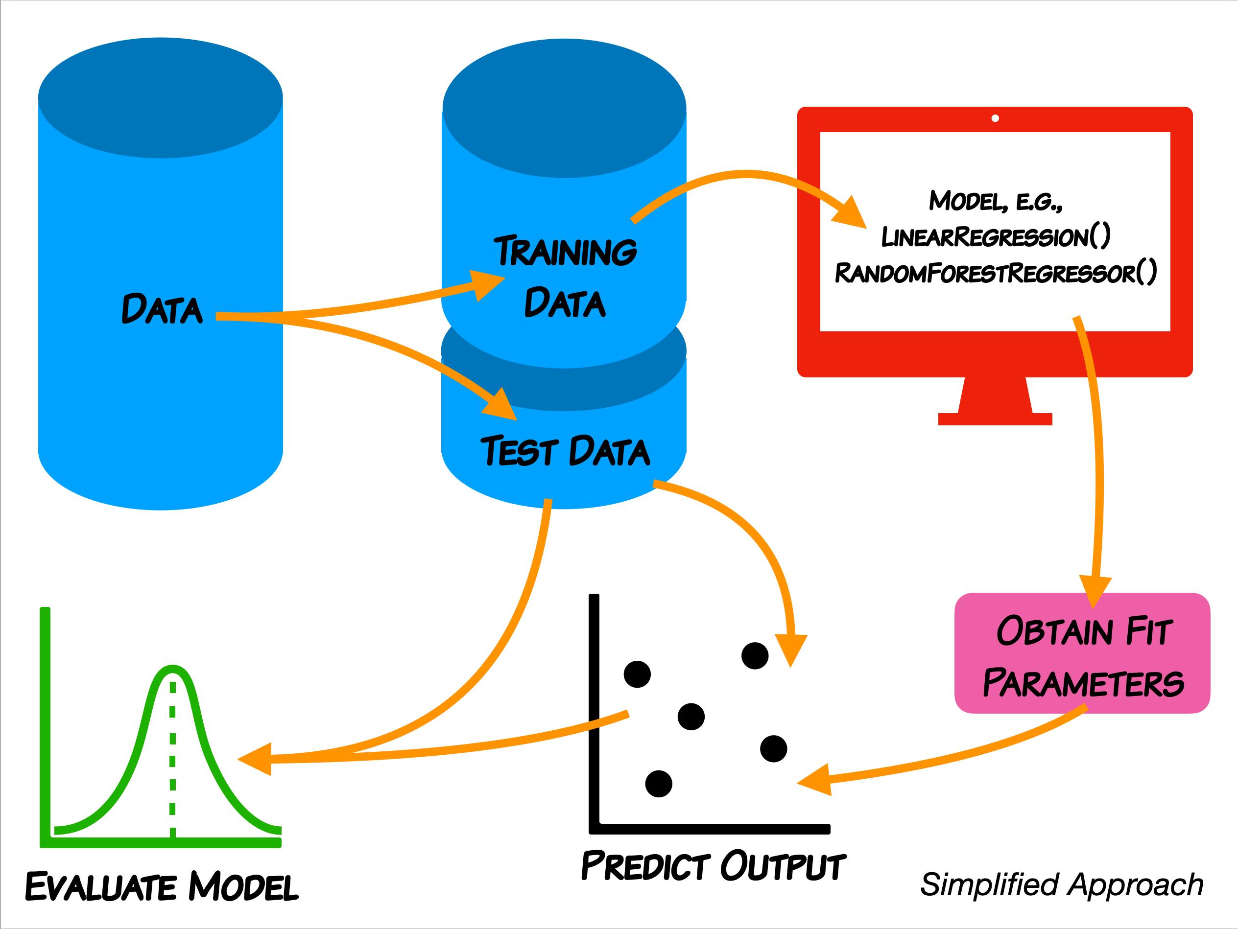
For this analysis, we will use the paradigm that we discussed where we split the data into a training set the develop the model and then use the model to predict the outcomes of a test set.
3.1 Splitting the data
We first need to split the data into a training set and a test set. To do this, we will also need to know which variable we intend to predict. The library sklearn has builtin methods for doing this splitting, so we will also need to import it. Notice that you can import a library any time that you need to.
Import
train_test_splitfromsklearn.model_selection.Look at your data and determine which columns will be the input features of your model and which will be the predicted variable. You might find using
columnsuseful. [Return column labels]Split the data into training and testing data sets using the
sklearn.model_selectionmethodtrain_test_split[How to use train_test_split]
Questions
How large is the training data set?
How can you change the amount of data used in the training set? [How to use train_test_split]
3.2 Creating and scoring the model
Now that we have split the data into training and test sets, we can build a model of the training set. We will focus first on a linear model using an ordinary least squares (OLS) fit. This is likely a model that you are familiar with, particularly for lines of best fit between two measurements. The general approach is to construct a linear model for student records that minimizes the error using OLS. to do this we need to import the LinearRegression method from sklearn.linear_model, then create a model, fit it, and score it. Notice: this approach to using linear regression with sci-kit learn is quite similar across other regression methods.
Import the
LinearRegressionmethod fromsklearn.linear_model[How to use LinearRegression]Create an OLS model and fit it.
Score the model using your model’s built in
scoremethod.
Questions
What does score represent? What is it summarizing? [The score method]
Are we justified in using a linear model? [Read about assumptions of linear models]
4. Analysing the model output
Now that we have established the goal of the model is to minimize the error, created a model, and found a score for the model, we still must recognize that the model has some error. The error/residual is really just the linear distance from the model “plane” to the predicted value as shown below:
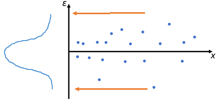
These residuals are data in their own right. But instead of being data about students, courses, etc. they are data about the model and how it is giving predictions. Thus we can use them to describe the model performance.
4.1 Predicting from test data
We will start by investigating how well our model, constructed from the training set, predicts the scores from test set.
Create predicted data using the model’s
predictmethod.Make a scatter plot to compare it to the actual values and draw a diagonal through this plot.
Questions
What “shape” does the scatter plot “blob” look like?
Does the “blob” follow the diagonal line or does it deviate in some way?
Can you tell if the model over or under predicts scores in the test set?
4.2 Inspecting the residuals of the model
One of the major assumptions of a linear model is that error is normall distributed. Basically, we aim for the error in the model to be distributed equally around zero, so that there’s little heteroscedasticity. If a linear model has errors that are not normally dsitributed, we are might be in a little be of trouble with regard to believing the model, and we might have to try another modeling approach. One way to look into this is to compute and plot the residuals. They should be roughly normally distributed if we are justfied in using a linear model. This analysis will tell us if our model tends to overpredict or underpredict scores and for which scores it does so.
Write a function to calculate the residuals of the model.
Plot the actual values versus the residuals using a scatter plot. (This is the most common way of seeing a residual analysis in practice.)
Collapse the residual scatter plot into a histogram. (This is a useful visualization to see the normality of the distribution) [How to plot a histogram]
Questions
Do we appear to be justified in using a linear model?
Does the model tend to overpredict or underpredict certain groups of scores?
5. Model Features - training and fitting
All models have some input data X and some output prediction Y. The input data X is of the shape \(m \times n\), so that means there are \(m\) columns (or features) and \(n\) data “points” (or vectors if \(m>1\)). For many models, you can return values from the model that give some indication as to how “important” each particular feature is to the model’s training. Typically, the larger the magnitude of this value, the more important the feature is for prediction. This value for linear models is called the model coefficients. It may also be called feature importance. These values are always calculated from the data that was used to train (fit) the model. Thus, they don’t really tell us about how important the features are for new data, rather how important the features were in deciding the “shape” of the model itself.
Finding fit coefficients
For our linear model, the coefficients are related to the correlation between each input varaiable and the output prediction. Earlier you looked at the correlations between each input variable and the output variable. Now, we return the linear fit coefficients and plots them to see which features are most “important” to our model. LinearRegression has a builtin attribute coef_ that returns these fit coefficients.
Return the fit coefficients using
coef_Make a bar graph of all the features in the model. [How to make a horizontal bar plot]
Questions
Which is the most important feature for fitting?
Which is least important?
6. Model Features - predicting
The correlary to each feature’s coefficient or importance value, is the amount of variance that feature explains in the prediction. Remember, we have split the data into two separate sets, the training data and the testing data. The test data is never shown to the model until after the model is “fit” to the training data. This secrecy is why we are able to test the predictive power of each model. This secret or “hold out” data can be used to measure the “explained variance” of each coefficient/feature. One method of doing this is called recursive feature elimination. Essentially, the coefficient of the model are ordered by magnitude, and the smallest are then removed one at a time until only one feature is left. Each iteration the model’s score function is called. This provides a ranking based on the predictive power of the features.
Finding the explained variance
Import
RFECVfromsklearn.feature_selection.Using the
RFEfunction, calculate the explained variance of each of the features in your model usinggrid_scores_. [How to use RFE]Plot the scores returned for each of the combination of features from largest contributions to smallest as a line plot.
Questions
What fraction of the variance is explained by the whole model?
Which input features explain the most variance?
Which explain the least and could be dropped in order to find a parsimonious model?
7. Other regressors
We used a linear model, but we could easily subsitute another regressor. Let try an algorithm called “Random Forest”. This algorithm has the ability to weight the features relative to each other. Let’s explore the residuals and the feature importances of the Random Forest algorithm.
Import the
RandomForestRegressormethod fromsklearn.ensemble[How to use RandomForestRegressor]Using your train dataset, create your Random Forest model and fit it.
7.1 Creating the model
7.2 Predicting from test data
Just like for the OLS model above, we will start by investigating how well our model, constructed from the training set, predicts the scores from test set.
Create predicted data using the model’s
predictmethod.Score the accuracy of your model by calculating the
mean_squared_errorbetween the predictions from your fit model and your test dataset outcomes.Make a scatter plot to compare it to the actual values and draw a diagonal through this plot.
Questions
What does the root mean squared error tell us? How does it compare to the
scorefrom the OLS model above?What “shape” does the scatter plot “blob” look like? How does it compare to the Linear Regression plot we made above?
Does the “blob” follow the diagonal line or does it deviate in some way?
Can you tell if the model over or under predicts scores in the test set?
7.3 Inspecting the residuals of the model
Write a function to calculate the residuals of the model.
Plot the actual values versus the residuals using a scatter plot. (This is the most common way of seeing a residual analysis in practice.)
Collapse the residual scatter plot into a histogram. (This is a useful visualization to see the normality of the distribution) [How to plot a histogram]
Questions
How does this plot compare to the plot we produced for Linear Regression?
Does the model tend to overpredict or underpredict certain groups of scores?
7.4 Finding feature importances
For our linear model above, the coefficients are related to the correlation between each input varaiable and the output prediction. Earlier you looked at the correlations between each input variable and the output variable. The Random Forest algorithm feature importances says that in a given model these features are most important in explaining the target variable. These importances are relative to each of the other features in your model.
Return the fit importances using
feature_importances_Make a bar graph of all the features in the model. [How to make a horizontal bar plot]
Questions
Which is the most important feature for fitting?
Which is least important?
How do this compare to the coefficients we analyzed in OLS model above?