Classification using K Nearest Neighbors
Contents
Classification using K Nearest Neighbors
Agenda for today
Review Gettting Started Assignment
Remind ourselves of Train vs Test
Use KNN classifier on breast cancer dataset
Evaluate the quality of the model
0. Imports for the day
import pandas as pd
import matplotlib.pyplot as plt
import numpy as np

from sklearn.model_selection import train_test_split
from sklearn.neighbors import KNeighborsClassifier
from sklearn import metrics

plt.style.use('ggplot')
%matplotlib inline
1. Review of Getting Started Notebook
Pull up the solution notebook
2. Training vs Testing
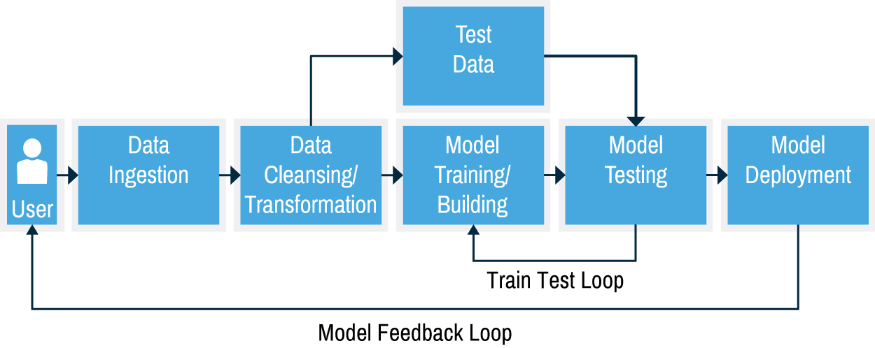
As you learned in the pre-class, classification is an ML process that maps features of an input data set to class labels. Classification is a supervised learning approach where example data is used to train the data. We typically divide the data used to train and evaluate the classifier (the result model) into two sets (training and testing). In some cases, folks split into three sets (training, testing, and validation).
✅ Do This: As a group, discuss what these three sets represent. It might help to review these terms on the web. The answers down below:
✎ Training set is:
✎ Testing set is:
Defining the features and building the model
If you review the image at the top of the notebook, you might notice that one of the first steps in machine learning is to go from “raw data” into a set of “features” and “labels”. Extracting features from our data can sometimes be one of the trickier parts of the process and also one of the most important ones. We have to think carefully about exactly what the “right” features are for training our machine learning algorithm and, when possible, it is advantageous to find ways to reduce the total number of features we are trying to model. Once we define our features, we can build our model.
2.1 Working with data
There is a common data set used to work with classification called the breast cancer data set. It is actually available in sklearn but what fun is working withe cleaned up data. Let’s look at the original. We will use data from a Breast Cancer study for this notebook. On this site, you will find “breast-cancer-wisconsin.data” and “breast-cancer-wisconsin.names”. The data are in “.data” and the “.names” describes that data.
We can also directly import them from the web:
Read in the data, label the columns based on the .names file. Look at the dtypes, anything unusual? Why?
✎ What’s unusual about dtypes? Why?
# your code here
Can you write code to identify what the problem is? That is, can you provide a DataFrame of the offending rows that are causing the problem? There are lots of ways to do this and, frankly, it is probably a bit hard so don’t get hung up too long on this. Give it a try though:
# your code here
OK, we have an imputation problem. Write code to solve it and say what you did.
By the way, there is an argument na_values that you can provide to read_csv that will mark a list of characters as if they were np.nan using na_values, which is pretty darn convenient. Using that will help when importing the data for classification.
Read the data in using na_values='?' to replace missing data with np.nan. Check the dtypes again.
# code here
2.2 : Splitting the dataset for model into training and testing sets
Let’s split the data in a training set and final testing set. We want to randomly select 75% of the data for training and 25% of the data for testing.
You should turn the class_labels into 0 (now 2, for benign) and 1 (now 4, for malignant) as the classifier we are using (Logisitic Regression) predicts valuse between 0 and 1.
✅ Do This - You will need to come up with a way to split the data into separate training and testing sets (we will leave the validation set out for now). Make sure you keep the feature vectors and classes together.
BIG HINT: This is a very common step in machine learning, and there exists a function to do this for you in the sklearn library called train_test_split. From the documentation, you find that takes the features and class labels as input and returns a 4 outputs:
2 feature sets (one for training and one for testing)
2 class labels sets (the corresponding one for training and for testing)
Use train_test_split to split your data into a training set and a testing set that correspond to 75% and 25% of your data respectively. Check the length of the resulting output to make sure the splits follow what you expected.
One last thing: KNN doesn’t work with missing data. You will need to use dropna() to get rid of them.
## your code here
Question: Why do we need to separate our samples into a training and testing set. Why can’t we just use all the data for both? Wouldn’t that make it work better?
✎ Do This - Erase the contents of this cell and replace it with your answer to the above question! (double-click on this text to edit this cell, and hit shift+enter to save the text)
3 K Nearest Neighbors
One of the more conceptually simply classifiers in K Nearest Neighbors or KNN. In KNN, we assume that in the N-dimensional space, which represents the N input features, that things in the same close are “close” to each other. That is the more similar their location in this virtual space, the more likely two points (or three or four…) are members of the same class.
KNN has one basic “hyperparameter”, which is what we can use to tune the model. It is how many neighbors it should include as part of the analysis (2, 3, 4, etc.). We will explore this at the end of the notebook. For now, we will setup the model.
More information on KNN from a conceptual persepctive is in the video below.
from IPython.display import YouTubeVideo
YouTubeVideo("HVXime0nQeI",width=640,height=360)
3.1 The benefits of sklearn
The sklearn workflow is similar across all implementations. We will always:
Create the model object (in this case
KNeighborsClassifier()). You can set hyperparameters at this step.Fit the model to the training data (this uses the
.fit()method).Use that model to predict from the test set (this uses the
.predict()method).
If you named your training and testing data: Xtrain, Xtest, ytrain, ytest, then this call is quite simple.
knn = KNeighborsClassifier()  ## Create model object
knn.fit(Xtrain,ytrain)        ## Fit model to training data
ypred = knn.predict(Xtest)    ## Predict the classes of the test data
✎ Do this. Implement this knn model for your data. What is ypred? What does ypred look like?
# your code
3.1 How’d it go?
There are a number of ways that we can check the performance of our model. The major difference in the standard statistics approach and supervised learning approaches is that we test our models using the data that we held out: “the test data.”
That is, we will use our classifier model to make predictions from the test features and we can then compare those predictions to actual test labels. As you did above, we can use the output of the .fit() method of the model to predict how well the classifier works on the test data (the data it was not trained on). Conveniently that is the .predict() method and, again, we use it on the result of the .fit().
But how well did the model do? It turns out that we can’t simply make a plot of predicted versus actual like we did for regression. Instead, we use the “confusion matrix” and associated measures derived from it. The Confusion Matrix gives you the number of true positives (TP), true negatives (TN), false positives (FP), and false negatives (FN). Through this we can determine the accuracy but the total number of TPs and TNs compared to all the data in the test set.
In the metrics library, there’s a method called confusion_matrix Documentation. We will start by using that.
✎ Using this method to print out the confusion matrix. What is the number of TPs, TNs, FPs, and FNs in your model? Can you calculate the accuracy (1 is perfect, 0 is terrible) of the model from these?
# your code here
This accuracy metric is alrady built into sklearn, it’s called accuracy_score, which compares the predictions our model made for the test labels and the actual test labels. The accuracy_score is one of many metrics we can use and is included in sklearn.metrics. Here’s the documentation on accuracy_score.
✎ Do this:
Use the
sklearn.metricswe imported at the top and run theaccuracy_scoreon the 0/1 predicted label and the test labels.Print your accuracy result
## your code here
Question: How well did your model predict the test class labels? Given what you learned in the pre-class assignment about false positives and false negatives, what other questions should we ask about the accuracy of our model?
✎ Answer here.
4. Tuning hyperparameters
Most ML models have some number of parameters that can be tuned to try to build better models. Later, we will see hwo to explore those parameters automatically, but now, we will just do things manually. For KNN, this is ok because there’s only one commnly tuned parameter: n_neighbors, which the number of neighboring points the algorithm takes into account when it looks for similar classes.
Look at the documentation for KNN and determine the default number of neighbors.
✎ Do this.
Repeat your analysis above (you only need to create a new model, not resplit the data!).
Choose a number of neighbors that is fewer than the default.
How does your model perform compared to the default?
## your code here
4.1 Automate it
Now that you have checked a slightly different number of neighbors, let’s systematically see how our accuract changes with number of neighbors.
✎ Do this.
Write a function that takes number of neighbors and returns accuracy of the model
For 2 to 10 neighbors, compute the accuracy
Plot the accuracy as a function of number of neighbors
What happens to the accuracy? Is there a good choice of n_neighbors to acheive the highest accuracy?
## your code here