Solution - Multidimensional Linear Regression¶

Goals¶

After completing this notebook, you will be able to:

Read in a fixed width data set and assign column names
Clean missing data from a data set
Construct a set of linear regression model usings scikit-learn
Evaluate the quality of fit for a set of models using adjusted \(R^2\) and by comparing true and predicted values
Explain why that model is the best fit for this data

0. Our imports¶

import numpy as np
import matplotlib.pyplot as plt
import pandas as pd

from IPython.display import HTML

from sklearn.model_selection import train_test_split
from sklearn.linear_model import LinearRegression
import sklearn.metrics as metrics

%matplotlib inline

1. Working with example data¶

We are going to work with some data generated by U.N.E.S.C.O. (United Nations Education, Scientific, and Cultural Organization) and data they collected relating to poverty and inequality in the world. There are two files you need to do the work:

poverty.dat which is the data file itself
poverty.txt which describes the data columns as fixed width column data. That is, this file describes the columns of the data for each category. For example, the data in columns 1-6 of poverty.dat contain the “live birth rates per 1,000 population”.

https://raw.githubusercontent.com/dannycab/MSU_REU_ML_course/main/notebooks/day-2/poverty.dat

https://raw.githubusercontent.com/dannycab/MSU_REU_ML_course/main/notebooks/day-2/poverty.txt

Conveniently there is a fixed width column pandas data reader called read_fwf (Documentation). You will need to specific column names also. No column headers appear in this data file, so look at the poverty.txt file and give them short but useful names.

✎ Do This - Read in the data into a DataFrame and print the head().

## your code here

### ANSWER ###

poverty_df = pd.read_fwf('https://raw.githubusercontent.com/dannycab/MSU_REU_ML_course/main/notebooks/day-2/poverty.dat', 
                         names = ['birth rate',
                                    'death rate',
                                    'infant mortality',
                                    'male LE',
                                    'female LE',
                                    'GNP',
                                    'country group',
                                    'country'])
poverty_df.head()

	birth rate	death rate	infant mortality	male LE	female LE	GNP	country group	country
0	24.7	5.7	30.8	69.6	75.5	600	1	Albania
1	12.5	11.9	14.4	68.3	74.7	2250	1	Bulgaria
2	13.4	11.7	11.3	71.8	77.7	2980	1	Czechoslovakia
3	12.0	12.4	7.6	69.8	75.9	*	1	Former_E._Germany
4	11.6	13.4	14.8	65.4	73.8	2780	1	Hungary

1.1 Type of the data¶

Now look at the .dtypes of your DataFrame and describe to me anything unusual. Can you explain why? Please write below. Don’t skimp and look ahead, think about it and answer! We’ll all wait ⏲

✎ Answer here

1.2 Handling missing data - Imputation¶

Let’s face it, sometimes data is bad. Values are not recorded, or are mis-recorded, or are so far out of expectation that you expect there is something wrong. On the other hand, just changing the data seems like cheating. We have to work with what we have, and if we have to make changes it would be good to do that programmatically so that it is recorded for others to see.

The process of imputation is the statistical replacement of missing/bad data with substitute values. We have that problem here. In the GNP column some of the values are set to ” * ” indicating missing data. When pandas read in the column the only type that makes sense for both characters and numbers is a string. Therefore it set the type to object instead of the expected int64 or float64.

Using numpy.nan¶

For better or worse, pandas assumes that “bad values” are marked in the data as numpy NaN. NaN is short for “Not a Number”. If they are so marked we have access to some of the imputation methods, replacing NaN with various values (mean, median, specific value, etc.).

There are two ways to do this:

you can do a .replace on the column using a dictionary of {value to replace : new value, …} pairs. Remember to save the result. This leaves you with changing the column type using .astype but you will have convert to a float, perhaps "float64" would be good. You cannot convert a np.nan to an integer but you can to a float.
you can convert the everything that can be converted to a number using .to_numeric. Conveniently if it can’t do the conversion on a particular value it is set to a np.nan

✎ Do This - Convert the missing entries in the GNP column to np.nan and show the head of your modified DataFrame. Also print the dtypes to show that the column has change type.

## your code here

### ANSWER ###

poverty_df['GNP'].replace(to_replace='*', value=np.nan, inplace=True)
poverty_df['GNP'] = poverty_df['GNP'].astype('float64')

poverty_df.dtypes

birth rate          float64
death rate          float64
infant mortality    float64
male LE             float64
female LE           float64
GNP                 float64
country group         int64
country              object
dtype: object

Changing numpy.nan¶

Now that “bad values” are marked as numpy.nan, we can use the DataFrame method fillna to change those values. For example:

## Uncomment to run

poverty_df["GNP"].fillna(0)

    600.0
   2250.0
   2980.0
      0.0
   2780.0
       ...  
   220.0
   110.0
   220.0
   420.0
   640.0
Name: GNP, Length: 97, dtype: float64

returns a new DataFrame where all the np.nan in the GNP column are replaced with 0. You can do other things are well, for example:

## Uncomment to run
poverty_df["GNP"].fillna(poverty_df["GNP"].mean() )
poverty_df.fillna({"GNP": poverty_df["GNP"].mean() })

	birth rate	death rate	infant mortality	male LE	female LE	GNP	country group	country
0	24.7	5.7	30.8	69.6	75.5	600.000000	1	Albania
1	12.5	11.9	14.4	68.3	74.7	2250.000000	1	Bulgaria
2	13.4	11.7	11.3	71.8	77.7	2980.000000	1	Czechoslovakia
3	12.0	12.4	7.6	69.8	75.9	5741.252747	1	Former_E._Germany
4	11.6	13.4	14.8	65.4	73.8	2780.000000	1	Hungary
...	...	...	...	...	...	...	...	...
92	52.2	15.6	103.0	49.9	52.7	220.000000	6	Uganda
93	50.5	14.0	106.0	51.3	54.7	110.000000	6	Tanzania
94	45.6	14.2	83.0	50.3	53.7	220.000000	6	Zaire
95	51.1	13.7	80.0	50.4	52.5	420.000000	6	Zambia
96	41.7	10.3	66.0	56.5	60.1	640.000000	6	Zimbabwe

97 rows × 8 columns

The first version changes any np.nan in the GNP column to be the mean of the column. The second takes a dictionary where the the key of the dictionary is the column to change and the value is what to replace the np.nan with. Note you could replace with other values like: median, min, max, or some other fixed value.

Remember that all of these examples return either a new Series (when working with just a column) or a DataFrame (if working with the entire element). Nothing is changed in the original unless you assign the result or use inplace=True in the call.

Finally, if you decide that the right thing to do is remove any row with a np.nan value, we can use the .dropna method of DataFrames as shown below:

## Uncomment to run
len(poverty_df)
poverty_df_dropped = poverty_df.dropna()
print(len(poverty_df), len(poverty_df_dropped))

97 91

What do you think¶

In the cell below, discuss with your group what you think is the best thing to do with the “bad values” in the DataFrame given the discussion above. Write your result below.

✎ Answer here

2. Multiple Regression¶

In the past, we have limited ourselves to either a single feature or, in the pre-class, doing polynomial regression with other features we created. However, we can just as easily use all, or some combination of all, the features available to make a OLS model. The question is, is it a good idea to just use all the possible features available to make a model?

Please discuss that idea with your group and record your answer below.

✎ Answer here

2.1 Infant Mortality model¶

Using the U.N.E.S.C.O. data, we can make a model of “Infant Mortality” as the dependent variable against all the other available features. As a hint, an easy way to do this is the make the model with “Infant Mortality” as the prediction (the dependent variable) and then the entire DataFrame where “Infant Mortality is dropped as the data (the independent variables). You should also drop the “Country” column as unique strings don’t play well in basic linear models.

✎ Do This - Make an linear model (did you split your data?) that predicts “Infant Mortality” using the other variables (dropping the “Country” column) and print the .r2_score of that process.

# your code here

### ANSWER ###

X = poverty_df_dropped.drop(columns = ['infant mortality', 'country'])
y = poverty_df_dropped['infant mortality']

X_train, X_test, y_train, y_test = train_test_split(X, y, test_size=0.2, random_state=42)

linear = LinearRegression()

linear.fit(X_train,y_train)

y_pred = linear.predict(X_test)

r2=metrics.r2_score(y_test, y_pred)
print('r2: ', round(r2,4))

r2:  0.9401

2.2 Visualizing your fit¶

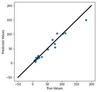
We can check how well we are justified in using this model, by comparing the actual and predicted values. Plot the predicted values against the real values. In a perfect model, they would form a line with a slope of 1.

✎ Do This - Make the plots mentioned above. How well does your model fit your data? What can you conclude from this graph?

### your code here

### ANSWER ###

plt.figure(figsize=(5,5))
plt.scatter(y_test,y_pred)
plt.xlabel('True Values')
plt.ylabel('Predicted Values')
plt.plot([-50,200],[-50,200], color='k', lw=3)

# res = y_test-y_pred

# plt.figure(figsize=(5,5))
# plt.scatter(X_test['male LE'], res)
# plt.xlabel('x')
# plt.ylabel('Residuals')

[<matplotlib.lines.Line2D at 0x165488cd0>]

../../_images/Day-2_Multiple_Regression-SOL_27_1.png

2.3 A “reduced” model using only the “significant” features¶

Modeling data is as much a craft as it is a science. We often seek the simplest models that explain or data well because they are typically more interpretable, easier to explain, and provide the information on the main influences of the system we are studying. There are reasons we might want a more complex model to capture the details and the nuance of the system. But for the U.N.E.S.C.O. data that we have, we are likely able to capture most of the system using a smaller number of features.

✎ Do This - use pandas built=in correlation function (.corr()) to find the top 3 variables that correlate strongly with “Infant Mortality”

# your code here

### ANSWER ###

poverty_df_dropped.corr()

	birth rate	death rate	infant mortality	male LE	female LE	GNP	country group
birth rate	1.000000	0.505626	0.856537	-0.866200	-0.894440	-0.629059	0.710212
death rate	0.505626	1.000000	0.677741	-0.754032	-0.714751	-0.302754	0.344168
infant mortality	0.856537	0.677741	1.000000	-0.935238	-0.954225	-0.601647	0.631913
male LE	-0.866200	-0.754032	-0.935238	1.000000	0.981957	0.642963	-0.642059
female LE	-0.894440	-0.714751	-0.954225	0.981957	1.000000	0.650040	-0.699097
GNP	-0.629059	-0.302754	-0.601647	0.642963	0.650040	1.000000	-0.283399
country group	0.710212	0.344168	0.631913	-0.642059	-0.699097	-0.283399	1.000000

✎ Do This - Redo the model with only the top three features you found above vs “Infant Mortality”. Print the .r2_score, how does it compare to the full model?

### your code here

### ANSWER ###

X1 = poverty_df_dropped.drop(columns = ['infant mortality', 'country', 'country group', 'GNP', 'death rate'])
y1 = poverty_df_dropped['infant mortality']

X_train1, X_test1, y_train1, y_test1 = train_test_split(X1, y1, test_size=0.2)

linear = LinearRegression()

linear.fit(X_train1,y_train1)

y_pred1 = linear.predict(X_test1)

r2=metrics.r2_score(y_test1, y_pred1)
print('r2: ', round(r2,4))

r2:  0.9061

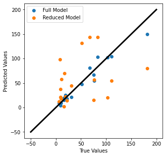
✎ Do This - Make the same comparison plot mentioned above. How well does your model fit your data? What can you conclude from this graph? Can you compare it to the previous fit?

### your code here

### ANSWER ###

plt.figure(figsize=(5,5))
plt.scatter(y_test,y_pred)
plt.scatter(y_test,y_pred1)
plt.xlabel('True Values')
plt.ylabel('Predicted Values')
plt.legend(['Full Model', 'Reduced Model'])

plt.plot([-50,200],[-50,200], color='k', lw=3)

# res = y_test-y_pred

# plt.figure(figsize=(5,5))
# plt.scatter(X_test['male LE'], res)
# plt.xlabel('x')
# plt.ylabel('Residuals')

[<matplotlib.lines.Line2D at 0x16557f4c0>]

../../_images/Day-2_Multiple_Regression-SOL_36_1.png

Review this model and the one you constructed earlier in the notebook. Report how the Adjusted R-squared value changed from using only the top three vs using all the available features. How well does this reduced model appear to fit your data?

✎ Answer here

2022 Oslo PER Summer Institute Machine Learning Short Course

Solution - Multidimensional Linear Regression

Contents

Solution - Multidimensional Linear Regression¶

Goals¶

0. Our imports¶

1. Working with example data¶

1.1 Type of the data¶

1.2 Handling missing data - Imputation¶

Using numpy.nan¶

Changing numpy.nan¶

What do you think¶

2. Multiple Regression¶

2.1 Infant Mortality model¶

2.2 Visualizing your fit¶

2.3 A “reduced” model using only the “significant” features¶